week-2-ml-mini-project

Analyzing govt. cost vs revenue (2015-16) using ml in octave

Obtaining data

The data used in the mini project was obtained from financial-performance-srtus-glance-2011-12-2015-16.

Cleaning data

The extra columns lie profit/loss and data of previous years was removed and the json file was converted to csv file having only the cost of 2015 and the revenue of 2015.

json file

data = {
  fields: [
    { id: "a", label: "S. No.", type: "string" },
    {
      id: "b",
      label: "Name of State Road Transport Undertaking (SRTU)",
      type: "string",
    },
    {
      id: "c",
      label: "Total Revenue (Rs. in Lakh) - 2015- 16",
      type: "string",
    },
    { id: "d", label: "Total Revenue (Rs. in Lakh) - 2014-15", type: "string" },
    { id: "e", label: "Total Cost (Rs. in Lakh) - 2015- 16", type: "string" },
    { id: "f", label: "Total Cost (Rs. in Lakh) - 2014-15", type: "string" },
    {
      id: "g",
      label: "Net Profit/Loss (Rs. in Lakh) - 2015- 16",
      type: "string",
    },
    {
      id: "h",
      label: "Net Profit/Loss (Rs. in Lakh) - 2014-15",
      type: "string",
    },
    {
      id: "i",
      label: "Profit before Tax (Rs. Lakh) - 2015- 16",
      type: "string",
    },
    {
      id: "j",
      label: "Profit before Tax (Rs. Lakh) - 2014-15",
      type: "string",
    },
  ],
  data: [
    [
      "1",
      "Ahmedabad MTC",
      "13039.7",
      "13028.54",
      "40690.58",
      "37684.7",
      "-27650.88",
      "-24656.16",
      "-26796.63",
      "-24527.08",
    ],
    [
      "2",
      "Andhra Pradesh SRTC",
      "501619.85",
      "400801.26",
      "556522.44",
      "444857.36",
      "-54902.59",
      "-44056.1",
      "-15020.1",
      "-12131.09",
    ]...

data = {
  fields: [
    { id: "a", label: "S. No.", type: "string" },
    {
      id: "b",
      label: "Name of State Road Transport Undertaking (SRTU)",
      type: "string",
    },
    {
      id: "c",
      label: "Total Revenue (Rs. in Lakh) - 2015- 16",
      type: "string",
    },
    { id: "d", label: "Total Revenue (Rs. in Lakh) - 2014-15", type: "string" },
    { id: "e", label: "Total Cost (Rs. in Lakh) - 2015- 16", type: "string" },
    { id: "f", label: "Total Cost (Rs. in Lakh) - 2014-15", type: "string" },
    {
      id: "g",
      label: "Net Profit/Loss (Rs. in Lakh) - 2015- 16",
      type: "string",
    },
    {
      id: "h",
      label: "Net Profit/Loss (Rs. in Lakh) - 2014-15",
      type: "string",
    },
    {
      id: "i",
      label: "Profit before Tax (Rs. Lakh) - 2015- 16",
      type: "string",
    },
    {
      id: "j",
      label: "Profit before Tax (Rs. Lakh) - 2014-15",
      type: "string",
    },
  ],
  data: [
    [
      "1",
      "Ahmedabad MTC",
      "13039.7",
      "13028.54",
      "40690.58",
      "37684.7",
      "-27650.88",
      "-24656.16",
      "-26796.63",
      "-24527.08",
    ],
    [
      "2",
      "Andhra Pradesh SRTC",
      "501619.85",
      "400801.26",
      "556522.44",
      "444857.36",
      "-54902.59",
      "-44056.1",
      "-15020.1",
      "-12131.09",
    ]...

converted csv file

40690.58,13039.7
556522.44,501619.85
5948.06,1746.18
16539.06,12380.43
251570.09,145377.74
219375.73,220748.39
11236.86,2487.18
39991.58,27375.44
20519.43,13405.27
570091.14,100498.79
281487.77,256695.66
190133.31,132416.16
92922.81,93095.39
9021.77,8711.06
...

40690.58,13039.7
556522.44,501619.85
5948.06,1746.18
16539.06,12380.43
251570.09,145377.74
219375.73,220748.39
11236.86,2487.18
39991.58,27375.44
20519.43,13405.27
570091.14,100498.79
281487.77,256695.66
190133.31,132416.16
92922.81,93095.39
9021.77,8711.06
...

Inputting data

One extra column of all ones was added to cost matrix for ease of computation

data = load("datafile.csv")
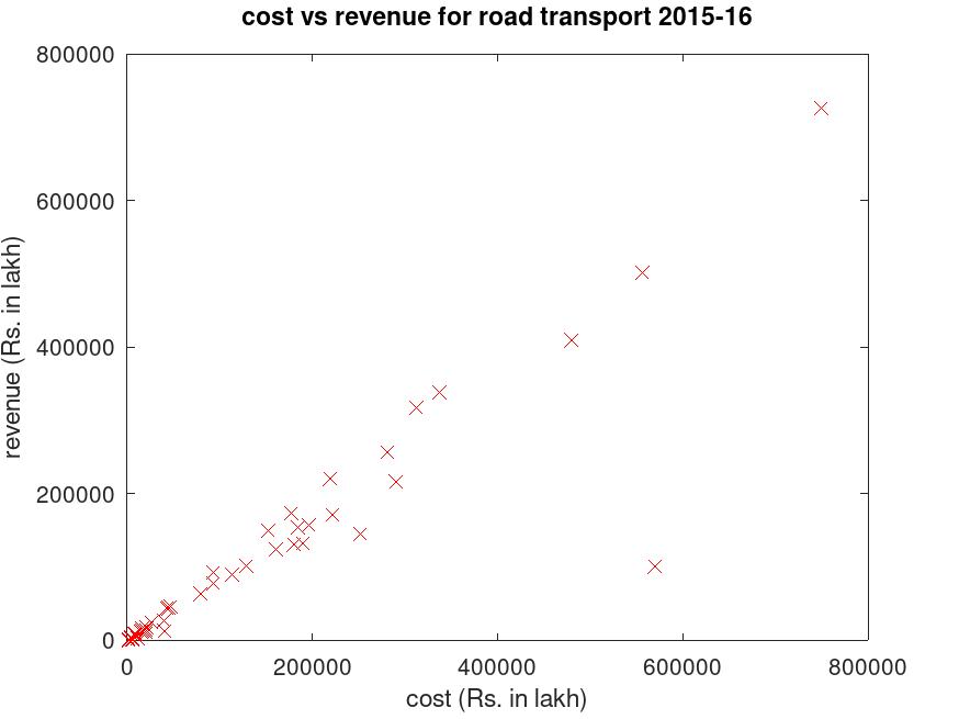
X = [ones(size(data)),data(:,1)]
y = data(:,2)

data = load("datafile.csv")
X = [ones(size(data)),data(:,1)]
y = data(:,2)

scatter plot of data

normalizing data

Following function was used for feature normalization of the data

function [X_norm, mu, sigma] = featureNormalize(X)
    mu = mean(X);
    sigma = std(X);
    X_norm = (X - mu)./sigma;

% normalized data
x_norm = featureNormalize(X)
x_norm(:,1) = ones(size(X),1)
y_norm = featureNormalize(y)

function [X_norm, mu, sigma] = featureNormalize(X)
    mu = mean(X);
    sigma = std(X);
    X_norm = (X - mu)./sigma;

% normalized data
x_norm = featureNormalize(X)
x_norm(:,1) = ones(size(X),1)
y_norm = featureNormalize(y)

values after feature normalization

X =
1.0000e+00   4.0691e+04
1.0000e+00   5.5652e+05
1.0000e+00   5.9481e+03
1.0000e+00   1.6539e+04
1.0000e+00   2.5157e+05
...

X =
1.0000e+00   4.0691e+04
1.0000e+00   5.5652e+05
1.0000e+00   5.9481e+03
1.0000e+00   1.6539e+04
1.0000e+00   2.5157e+05
...

Calculating graient descent

function [theta, J_history] = gradientDescent(X, y, theta, alpha, num_iters)
    %GRADIENTDESCENT Performs gradient descent to learn theta
    %   theta = GRADIENTDESCENT(X, y, theta, alpha, num_iters) updates theta by 
    %   taking num_iters gradient steps with learning rate alpha

    % Initialize some useful values
    m = length(y); % number of training examples
    J_history = zeros(num_iters, 1);

    for iter = 1:num_iters
        summation = sum((X*theta - y).*X);
        theta = theta - alpha * (summation/m)';

        % Save the cost J in every iteration    
        J_history(iter) = computeCost(X, y, theta);

    end

end



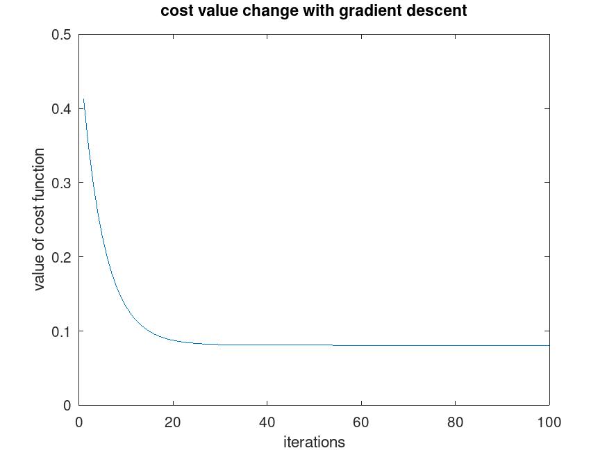
theta=[0;0]
[theta, j_history] = gradientDescent(x_norm,y_norm,theta,0.1,100)
plot(j_history )

function [theta, J_history] = gradientDescent(X, y, theta, alpha, num_iters)
    %GRADIENTDESCENT Performs gradient descent to learn theta
    %   theta = GRADIENTDESCENT(X, y, theta, alpha, num_iters) updates theta by 
    %   taking num_iters gradient steps with learning rate alpha

    % Initialize some useful values
    m = length(y); % number of training examples
    J_history = zeros(num_iters, 1);

    for iter = 1:num_iters
        summation = sum((X*theta - y).*X);
        theta = theta - alpha * (summation/m)';

        % Save the cost J in every iteration    
        J_history(iter) = computeCost(X, y, theta);

    end

end



theta=[0;0]
[theta, j_history] = gradientDescent(x_norm,y_norm,theta,0.1,100)
plot(j_history )

change in cost function depicting gradient descent

value of theta

theta =
  -1.3570e-16
   9.1355e-01

theta =
  -1.3570e-16
   9.1355e-01

Plotting regression line

%plotting original graph
plot(X(:,2),y,"rx")
%retaining previous graph
hold on
%plotting regressing line on top
plot(X,X*theta)

% calculating average loss
mux=mean(X(:,2))
muy=mean(y)
(mux-muy)/mux
((mux-muy)/mux)*100
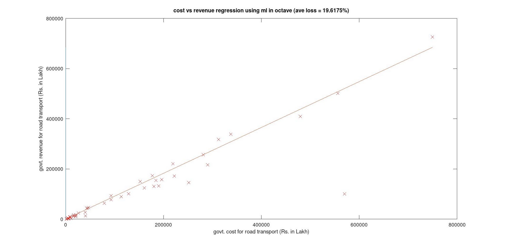
ave_loss = ((mux-muy)/mux)*100

% formatting graph
title("cost vs revenue regression using ml in octave (ave loss = 19.6175%)")
ylabel("govt. revenue for road transport (Rs. in Lakh)")
xlabel("govt. cost for road transport (Rs. in Lakh)")

%plotting original graph
plot(X(:,2),y,"rx")
%retaining previous graph
hold on
%plotting regressing line on top
plot(X,X*theta)

% calculating average loss
mux=mean(X(:,2))
muy=mean(y)
(mux-muy)/mux
((mux-muy)/mux)*100
ave_loss = ((mux-muy)/mux)*100

% formatting graph
title("cost vs revenue regression using ml in octave (ave loss = 19.6175%)")
ylabel("govt. revenue for road transport (Rs. in Lakh)")
xlabel("govt. cost for road transport (Rs. in Lakh)")

regression line along with data points

Conclusion

I had a lot of fun creating this mini project. Although the result was quite obvious from the beginning, still I wanted to apply what little I have learned on real data. I aspire to create many more such mini projects.